One-way ANOVA in SPSS Statistics
Introduction
The one-way analysis of variance (ANOVA) is used to determine
whether there are any significant differences between the means of two
or more independent (unrelated) groups (although you tend to only see it
used when there are a minimum of three, rather than two groups). For
example, you could use a one-way ANOVA to understand whether exam
performance differed based on test anxiety levels amongst students,
dividing students into three independent groups (e.g., low, medium and
high-stressed students). Also, it is important to realize that the
one-way ANOVA is an omnibus test statistic and cannot tell you
which specific groups were significantly different from each other; it
only tells you that at least two groups were different. Since you may
have three, four, five or more groups in your study design, determining
which of these groups differ from each other is important. You can do
this using a post-hoc test (N.B., we discuss post-hoc tests later in
this guide).
NOTE: If your study
design not only involves one dependent variable and one independent
variable, but also a third variable (known as a "covariate") that you
want to "statistically control", you may need to perform an ANCOVA
(analysis of covariance), which can be thought of as an extension of the
one-way ANOVA. To learn more, see our SPSS Statistics guide on ANCOVA. Alternatively, if your dependent variable is the time until an event happens, you might need to run a Kaplan-Meier analysis.
This "quick start" guide shows you how to carry out a one-way ANOVA
using SPSS Statistics, as well as interpret and report the results from
this test. Since the one-way ANOVA is often followed up with post-hoc
tests, we also show you how to carry out these using SPSS Statistics.
However, before we introduce you to this procedure, you need to
understand the different assumptions that your data must meet in order
for a one-way ANOVA to give you a valid result. We discuss these
assumptions next.
Assumptions
When you choose to analyse your data using a one-way ANOVA, part of
the process involves checking to make sure that the data you want to
analyse can actually be analysed using a one-way ANOVA. You need to do
this because it is only appropriate to use a one-way ANOVA if your data
"passes" six assumptions that are required for a one-way ANOVA to give
you a valid result. In practice, checking for these six assumptions just
adds a little bit more time to your analysis, requiring you to click a
few more buttons in SPSS Statistics when performing your analysis, as
well as think a little bit more about your data, but it is not a
difficult task.
Before we introduce you to these six assumptions, do not be
surprised if, when analysing your own data using SPSS Statistics, one or
more of these assumptions is violated (i.e., is not met). This is not
uncommon when working with real-world data rather than textbook
examples, which often only show you how to carry out a one-way ANOVA
when everything goes well! However, don’t worry. Even when your data
fails certain assumptions, there is often a solution to overcome this.
First, let’s take a look at these six assumptions:
- Assumption #1: Your dependent variable should be measured at the interval or ratio level (i.e., they are continuous). Examples of variables that meet this criterion include revision time (measured in hours), intelligence (measured using IQ score), exam performance (measured from 0 to 100), weight (measured in kg), and so forth. You can learn more about interval and ratio variables in our article: Types of Variable.
- Assumption #2: Your independent variable should consist of two or more categorical, independent groups. Typically, a one-way ANOVA is used when you have three or more categorical, independent groups, but it can be used for just two groups (but an independent-samples t-test is more commonly used for two groups). Example independent variables that meet this criterion include ethnicity (e.g., 3 groups: Caucasian, African American and Hispanic), physical activity level (e.g., 4 groups: sedentary, low, moderate and high), profession (e.g., 5 groups: surgeon, doctor, nurse, dentist, therapist), and so forth.
- Assumption #3: You should have independence of observations, which means that there is no relationship between the observations in each group or between the groups themselves. For example, there must be different participants in each group with no participant being in more than one group. This is more of a study design issue than something you can test for, but it is an important assumption of the one-way ANOVA. If your study fails this assumption, you will need to use another statistical test instead of the one-way ANOVA (e.g., a repeated measures design). If you are unsure whether your study meets this assumption, you can use our Statistical Test Selector, which is part of our enhanced guides.
- Assumption #4: There should be no significant outliers. Outliers are simply single data points within your data that do not follow the usual pattern (e.g., in a study of 100 students' IQ scores, where the mean score was 108 with only a small variation between students, one student had a score of 156, which is very unusual, and may even put her in the top 1% of IQ scores globally). The problem with outliers is that they can have a negative effect on the one-way ANOVA, reducing the validity of your results. Fortunately, when using SPSS Statistics to run a one-way ANOVA on your data, you can easily detect possible outliers. In our enhanced one-way ANOVA guide, we: (a) show you how to detect outliers using SPSS Statistics; and (b) discuss some of the options you have in order to deal with outliers. You can learn more about our enhanced one-way ANOVA guide here.
- Assumption #5: Your dependent variable should be approximately normally distributed for each category of the independent variable. We talk about the one-way ANOVA only requiring approximately normal data because it is quite "robust" to violations of normality, meaning that assumption can be a little violated and still provide valid results. You can test for normality using the Shapiro-Wilk test of normality, which is easily tested for using SPSS Statistics. In addition to showing you how to do this in our enhanced one-way ANOVA guide, we also explain what you can do if your data fails this assumption (i.e., if it fails it more than a little bit). Again, you can learn more here.
- Assumption #6: There needs to be homogeneity of variances. You can test this assumption in SPSS Statistics using Levene's test for homogeneity of variances. If your data fails this assumption, you will need to not only carry out a Welch ANOVA instead of a one-way ANOVA, which you can do using SPSS Statistics, but also use a different post-hoc test. In our enhanced one-way ANOVA guide, we (a) show you how to perform Levene’s test for homogeneity of variances in SPSS Statistics, (b) explain some of the things you will need to consider when interpreting your data, and (c) present possible ways to continue with your analysis if your data fails to meet this assumption, including running a Welch ANOVA in SPSS Statistics instead of a one-way ANOVA, and a Games-Howell test instead of a Tukey post-hoc test (learn more here).
You can check assumptions #4, #5 and #6 using SPSS Statistics. Before
doing this, you should make sure that your data meets assumptions #1, #2
and #3, although you don't need SPSS Statistics to do this. When moving
on to assumptions #4, #5 and #6, we suggest testing them in this order
because it represents an order where, if a violation to the assumption
is not correctable, you will no longer be able to use a one-way ANOVA
(although you may be able to run another statistical test on your data
instead). Just remember that if you do not run the statistical tests on
these assumptions correctly, the results you get when running a one-way
ANOVA might not be valid. This is why we dedicate a number of sections
of our enhanced one-way ANOVA guide to help you get this right. You can
find out about our enhanced one-way ANOVA guide here, or more generally, our enhanced content as a whole here.
In the section, Procedure,
we illustrate the SPSS Statistics procedure to perform a one-way ANOVA
assuming that no assumptions have been violated. First, we set out the
example we use to explain the one-way ANOVA procedure in SPSS
Statistics.
Example
A manager wants to raise the productivity at his company by increasing the speed at which his employees can use a particular spreadsheet program. As he does not have the skills in-house, he employs an external agency which provides training in this spreadsheet program. They offer 3 courses: a beginner, intermediate and advanced course. He is unsure which course is needed for the type of work they do at his company, so he sends 10 employees on the beginner course, 10 on the intermediate and 10 on the advanced course. When they all return from the training, he gives them a problem to solve using the spreadsheet program, and times how long it takes them to complete the problem. He then compares the three courses (beginner, intermediate, advanced) to see if there are any differences in the average time it took to complete the problem.SPSS Statisticstop ^
Setup in SPSS Statistics
In SPSS Statistics, we separated the groups for analysis by creating a grouping variable called Course (i.e., the independent variable), and gave the beginners course a value of "1", the intermediate course a value of "2" and the advanced course a value of "3". Time to complete the set problem was entered under the variable name Time (i.e., the dependent variable). In our enhanced one-way ANOVA guide, we show you how to correctly enter data in SPSS Statistics to run a one-way ANOVA (see here). You can learn about our enhanced data setup content in general here. Alternately, we have a generic, "quick start" guide to show you how to enter data into SPSS Statistics, available here.SPSS Statisticstop ^
Test Procedure in SPSS Statistics
The eight steps below show you how to analyse your data using a one-way ANOVA in SPSS Statistics when the six assumptions in the previous section, Assumptions, have not been violated. At the end of these eight steps, we show you how to interpret the results from this test. If you are looking for help to make sure your data meets assumptions #4, #5 and #6, which are required when using a one-way ANOVA, and can be tested using SPSS Statistics, you can learn more here.-
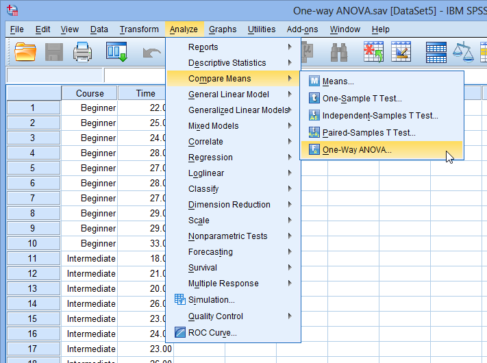
Click Analyze > Compare Means > One-Way ANOVA... on the top menu as shown below.
 Published with written permission from SPSS Statistics, IBM Corporation.
-
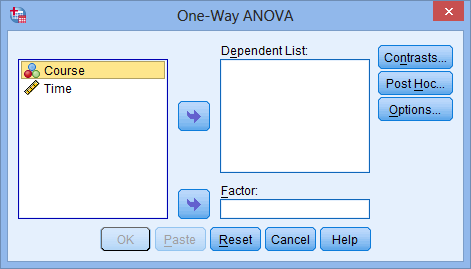
You will be presented with the following screen:
 Published with written permission from SPSS Statistics, IBM Corporation.
-
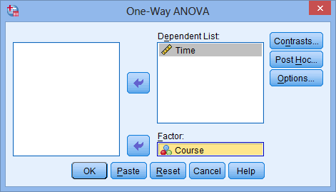
Transfer the dependent variable (Time) into the Dependent List: box and the independent variable (Course) into the Factor: box using the appropriate
 buttons (or drag-and-drop the variables into the boxes), as indicted in the diagram below:
 Published with written permission from SPSS Statistics, IBM Corporation.
-
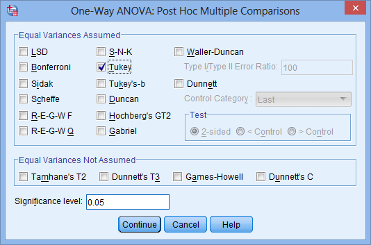
Click the
 button. Tick the Tukey checkbox as shown below:
 Published with written permission from SPSS Statistics, IBM Corporation.
-
Click the
 button.
-
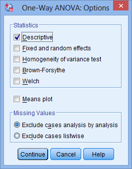
Click the
 button. Tick the Descriptive checkbox in the –Statistics– area, as shown below:
 Published with written permission from SPSS Statistics, IBM Corporation.
NOTE: When testing for some of the assumptions of the one-way ANOVA, you will need to tick more of these checkboxes. We take you through this, including how to interpret the output, in our enhanced one-way ANOVA guide. -
Click the button.
-
Click the
 button.
SPSS Statistics Output of the one-way ANOVA
SPSS Statistics generates quite a few tables in its one-way ANOVA analysis. In this section, we show you only the main tables required to understand your results from the one-way ANOVA and Tukey post-hoc tests. For a complete explanation of the output you have to interpret when checking your data for the six assumptions required to carry out a one-way ANOVA. This includes relevant boxplots, and output from your Shapiro-Wilk test for normality and test for homogeneity of variances. Also, if your data failed the assumption of homogeneity of variances, we take you through the results for Welch ANOVA, which you will have to interpret rather than the standard one-way ANOVA in this guide. Below, we focus on the descriptives table, as well as the results for the one-way ANOVA and Tukey post-hoc test only. We will go through each table in turn.Descriptives Table
The descriptives table (see below) provides some very useful descriptive statistics, including the mean, standard deviation and 95% confidence intervals for the dependent variable (Time) for each separate group (Beginners, Intermediate and Advanced), as well as when all groups are combined (Total). These figures are useful when you need to describe your data.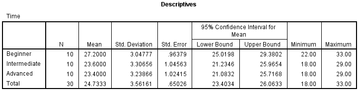 Published with written permission from SPSS Statistics, IBM Corporation.
ANOVA Table
This is the table that shows the output of the ANOVA analysis and whether we have a statistically significant difference between our group means. We can see that the significance level is 0.021 (p = .021), which is below 0.05. and, therefore, there is a statistically significant difference in the mean length of time to complete the spreadsheet problem between the different courses taken. This is great to know, but we do not know which of the specific groups differed. Luckily, we can find this out in the Multiple Comparisons table which contains the results of post-hoc tests.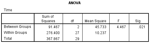 Published with written permission from SPSS Statistics, IBM Corporation.
Multiple Comparisons Table
From the results so far, we know that there are significant differences between the groups as a whole. The table below, Multiple Comparisons, shows which groups differed from each other. The Tukey post-hoc test is generally the preferred test for conducting post-hoc tests on a one-way ANOVA, but there are many others. We can see from the table below that there is a significant difference in time to complete the problem between the group that took the beginner course and the intermediate course (p = 0.046), as well as between the beginner course and advanced course (p = 0.034). However, there were no differences between the groups that took the intermediate and advanced course (p = 0.989).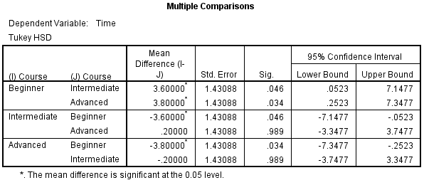 Published with written permission from SPSS Statistics, IBM Corporation.
SPSS Statisticstop ^
Reporting the output of the one-way ANOVA
Based on the results above, we could report the results of the study as follows (N.B., this does not include the results from your assumptions tests or effect size calculations):- General
There was a statistically significant difference between groups as determined by one-way ANOVA (F(2,27) = 4.467, p
= .021). A Tukey post-hoc test revealed that the time to complete the
problem was statistically significantly lower after taking the
intermediate (23.6 ± 3.3 min, p = .046) and advanced (23.4 ± 3.2 min, p
= .034) course compared to the beginners course (27.2 ± 3.0 min). There
were no statistically significant differences between the intermediate
and advanced groups (p = .989).
All thanks to LAERD STATISTICS


No comments:
Post a Comment